bmlm: Tutorial with Relationship Satisfaction Data
Matti Vuorre
2023-09-26
Source:vignettes/bmlm-blch9/bmlm-blch9.Rmd
bmlm-blch9.RmdIntroduction
bmlm is an R package that allows easy estimation of multilevel mediation models. bmlm uses the RStan interface to the powerful Stan Bayesian inference engine (Stan Development Team, 2016). Users can estimate, summarize and plot a multilevel mediation model easily with the convenient functions provided with bmlm. This document explains how to install bmlm and its required components, and then walks through an example of how to use it in practice.
Installing bmlm
Please ensure you have the latest version of R installed (R Core Team, 2016). The latest stable version of bmlm is available on CRAN:
install.packages("bmlm")Development version.
The latest development version of bmlm is available
on GitHub. The development
version sometimes has features that have not yet made it to the package
on CRAN. To install R packages from GitHub, please install the
devtools package first, as shown by the first line below.
Then install bmlm using devtools:
install.packages("devtools")
# Install from GitHub using the devtools package
devtools::install_github("mvuorre/bmlm", args = "--preclean")
If something goes wrong during the installation process, you will receive a notice usually asking you to install additional packages. If you are unable to resolve the problems, please open an issue on GitHub.
Example
After installing the required software, load the bmlm package to your current R workspace:
bmlm contains an example data set from Intensive Longitudinal Methods: An Introduction to Diary and Experience Sampling Research (Bolger & Laurenceau, 2013). We’ll use this data set in this example, and first load it into the workspace from the package, and display what the data looks like:
head(BLch9)## id time fwkstrs fwkdis freldis x m y
## 1 101 1 3 5.590119 3.034483 0.3333333 0.9828781 -1.4420726
## 2 101 2 3 5.535224 4.620690 0.3333333 0.9279833 0.1441343
## 3 101 3 3 3.888381 2.850575 0.3333333 -0.7188603 -1.6259807
## 4 101 4 4 5.352242 6.398467 1.3333333 0.7450007 1.9219121
## 5 101 5 1 4.483074 2.544061 -1.6666667 -0.1241668 -1.9324941
## 6 101 6 2 3.339433 5.164751 -0.6666667 -1.2678081 0.6881956Data preprocessing
The goal of multilevel mediation modeling, in this case, is to assess
the within-person relationships between X, M and Y. To this
end, it is important to isolate the within- and between-person
components of X, M, and Y. The isolate() function in
bmlm allows the user to create within- and
between-person centered values of variables. The example dataset
BLch9 already contains subject-mean deviated components,
but here we illustrate how to obtain these using the
isolate() function. The key inputs to this function are
d, a data frame; by a column of values that
identifies individuals; and value, which variable(s) should
be transformed.
head(BLch9)## id time fwkstrs fwkdis freldis x m y
## 1 101 1 3 5.590119 3.034483 0.3333333 0.9828781 -1.4420726
## 2 101 2 3 5.535224 4.620690 0.3333333 0.9279833 0.1441343
## 3 101 3 3 3.888381 2.850575 0.3333333 -0.7188603 -1.6259807
## 4 101 4 4 5.352242 6.398467 1.3333333 0.7450007 1.9219121
## 5 101 5 1 4.483074 2.544061 -1.6666667 -0.1241668 -1.9324941
## 6 101 6 2 3.339433 5.164751 -0.6666667 -1.2678081 0.6881956
## fwkstrs_cw fwkdis_cw freldis_cw
## 1 0.3333333 0.9828781 -1.4420726
## 2 0.3333333 0.9279833 0.1441343
## 3 0.3333333 -0.7188603 -1.6259807
## 4 1.3333333 0.7450007 1.9219121
## 5 -1.6666667 -0.1241668 -1.9324941
## 6 -0.6666667 -1.2678081 0.6881956The ..._cw variables now contain isolated within-person
(“subject-mean deviated”) pieces of each variable. We’ll use these for
the mediation analysis.
Fit model
To estimate the multilevel mediation model, run mlm()
and save its output to an object. Here we’ll call it fit.
You can also ask Stan to run multiple MCMC chains in parallel (if
supported by your computer).
fit <- mlm(d = BLch9,
           id = "id",
           x = "fwkstrs_cw",
           m = "fwkdis_cw",
           y = "freldis_cw",
           iter = 2000,
           cores = 4)
The main arguments to mlm() are d (a
data.frame), which here was set to BLch9. The
user also needs to specify which columns contain the variables needed
for the mediation model, unless they are already named id,
x, m, and y:
-
idis a column of participant IDs in the provideddata.frame. -
xis the manipulated variable. -
mis the mediator variable. -
yis the outcome variable.
There are various additional arguments to the above command. Most
notably, the iter = 2000 specified the number of samples to
draw from the posterior distribution, for each MCMC chain. The default
is to use 4 chains. Further, Stan’s MCMC algorithms use a portion of the
samples as warmup to adjust various underlying parameters. The default
of one half was used for this example.
Stan’s MCMC procedures are very efficient, but estimating the model with large datasets will take a while. This example takes about 30 seconds on a desktop Mac (8GB RAM, 4ghz Intel i7).
Summarize fitted model
After the samples have been obtained, bmlm’s helper functions can be used to obtain summaries of the results. For more options, all rstan methods are also available.
Numerical summary
A numerical summary of the “fixed” effects can be obtained by
mlm_summary(fit):
mlm_summary(fit)## Parameter Mean SE Median 2.5% 97.5% n_eff Rhat
## 1 a 0.19 0.04 0.19 0.12 0.26 5325 1
## 2 b 0.15 0.03 0.15 0.09 0.21 4559 1
## 3 cp 0.10 0.02 0.10 0.06 0.15 5019 1
## 4 me 0.06 0.01 0.06 0.03 0.09 1949 1
## 5 c 0.16 0.03 0.16 0.11 0.21 4450 1
## 6 pme 0.36 0.08 0.35 0.21 0.52 2420 1mlm_summary() returns, for each parameter, the following
information:
- Posterior Mean: This can be used as a point estimate of parameter
- SE: The standard deviation of the marginal posterior distribution of plausible parameter values.
- Posterior Median: If the posterior distribution is skewed, the median might be used as a more accurate point estimate.
- Lower and upper limits to Credible Intervals. The CIs
summarize the central X% mass of the marginal posterior distribution,
where X% is defined by a
levelargument tomlm_summary(). The default “confidence level” is 0.95, but users may supply any value they desire. - n_eff and Rhat are diagnostic values used to diagnose the
performance of the underlying Stan MCMC procedures. see
?mlmor?stanfor details.
Graphical summaries
bmlm provides functions for graphical summaries of
the estimated model. The first draws a path diagram of the mediation
model, with point estimates of the relevant average-level parameters,
and their associated credible intervals (as defined by
level). By default, the plot also shows the standard
deviations (SD) of the Gaussian distributions of the subject-level
varying effects, and their associated CIs. You can turn off the “random”
effects by calling the function with random = FALSE.
mlm_path_plot(fit, level = .95, text = T,
              xlab = "Work\nstressors",
              mlab = "Work\ndissatisfaction",
              ylab = "Relationship\ndissatisfaction", digits = 2)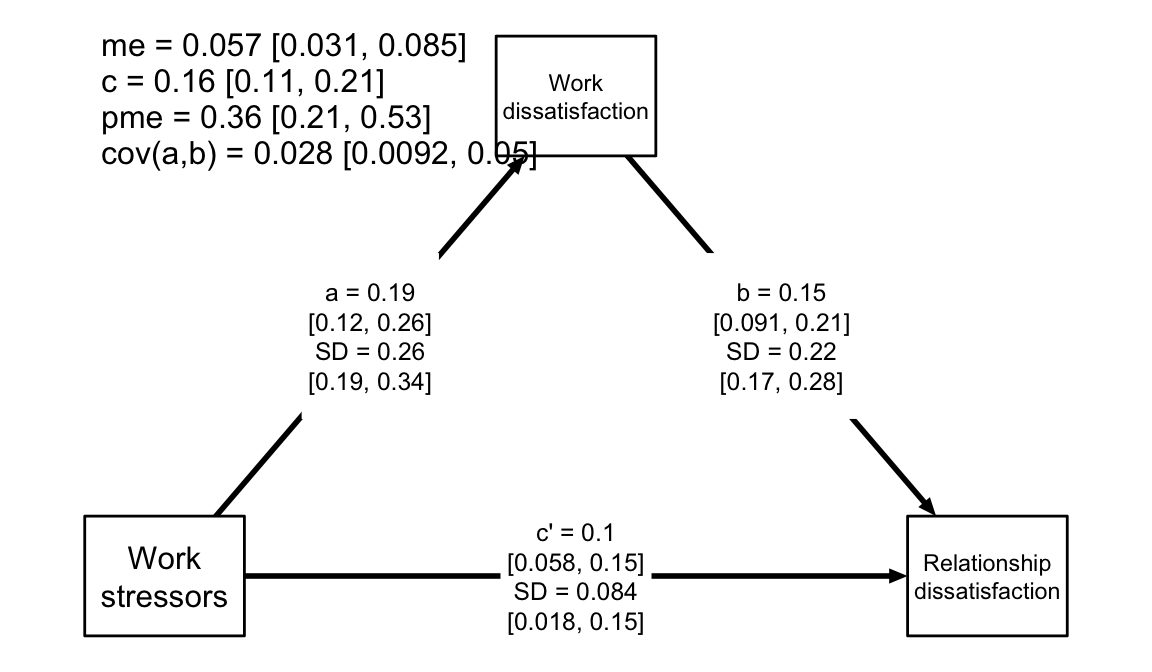
Path diagram of the average level mediation model, with numerical summaries of the relevant parameters.
This figure offers a quick view of the estimated model: All paths
(a, b, c') are positive with fairly narrow credible
intervals. However, the SD parameters indicate considerable
heterogeneity in the effects.
We called the function with the argument text = T,
showing additional transformed parameters in the upper left corner:
me is the average mediated effect, c is the
total effect, and pme is the proportion mediated effect.
cov(a, b) is the covariance of the varying a
and b parameters. To disable showing the additional
parameters, call the function with text = F.
For a more detailed investigation of the model’s parameters,
bmlm offers three methods for plotting the samples from
each parameter’s posterior distribution. These are obtained by a call to
mlm_pars_plot(type = X) where X can be either
hist (or left blank) for histograms, coef for
a coefficient plot with point estimates and Credible Intervals, or
“violin” for a violin plot. With coefficient plots, the user may specify
level to set the “confidence level”, which is represented
by the length of the lines surrounding each point estimate.
mlm_pars_plot(fit, pars = "me")
mlm_pars_plot(fit, type = "coef", level = .99)
mlm_pars_plot(fit, type = "violin", color = "dodgerblue2")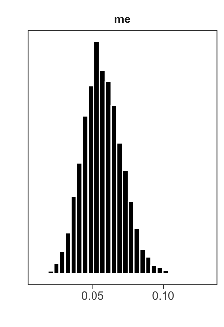
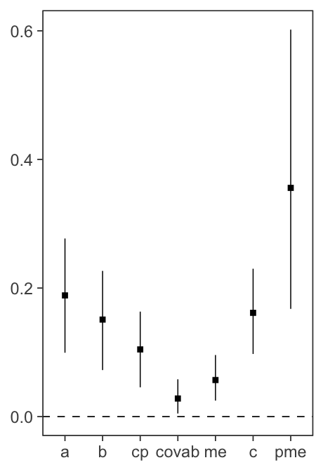
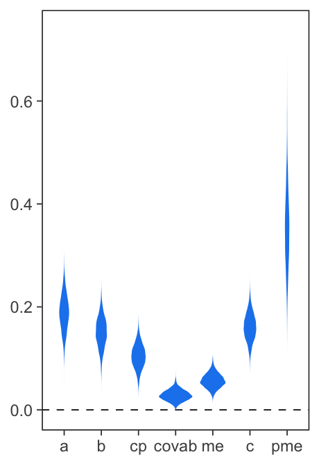
Figure 2. Coefficient plots.
The user can also specify the parameters to show on the plot, as illustrated in the next histograms:
mlm_pars_plot(fit, type = "hist", pars = c("me", "c", "pme", "covab"))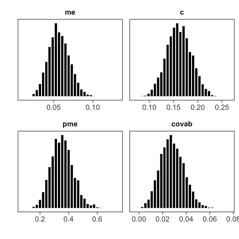
Histograms for a selection of parameters.
The histograms are useful for visually assessing the shape of each marginal posterior distribution.
More complex plots are also possible:
mlm_pars_plot(fit, type = "hist", pars = c(
    "tau_cp", "Omega[1,2]", "Omega[1,3]",
    "Omega[2,1]", "tau_b", "Omega[2,3]",
    "Omega[3,1]", "Omega[3,2]", "tau_a"),
    nrow = 3, color = "skyblue4")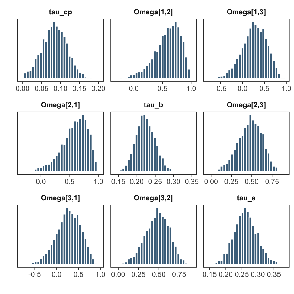
Varying effects standard deviations (tau) and correlations (Omega).
The first three positions (1: path c', 2: path
b, 3: path a) of the varying effects SDs
(\(\tau\)) and correlations (\(\Omega\)) are plotted as histograms. Each
histogram represents the MCMC samples of plausible parameter values from
the corresponding posterior distribution. These parameters are also
found with their names in the posterior samples matrix:
mlm_pars_plot(fit, pars = c("tau_a", "tau_b", "tau_cp",
                            "corrab"), nrow=2, color="dodgerblue2")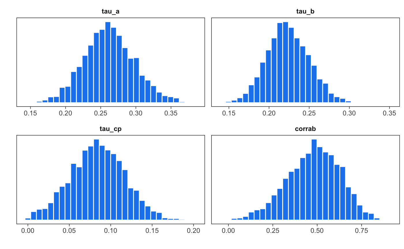
Plotting fitted values
Users can plot fitted values of the a and b paths, at the population
(fixed) and subject (random) levels, using
mlm_spaghetti_plot(). This function requires the user to
input a fitted multilevel mediation model object (mod), the
data used to fit the model (d), and the names of x, m, and
y variables that were used from the data.
ps <- mlm_spaghetti_plot(mod = fit, d = BLch9,
                         x = "fwkstrs_cw",
                         m = "fwkdis_cw",
                         y = "freldis_cw")
ps now contains a list of two plot objects. The first
plot contains the fitted values of the X -> M regression (path a). By
default, both the population- and subject-level fitted values are
included in the plot (see ?mlm_spaghetti_plot for how to
modify this behavior), the former is shown as a thicker line with a 95%
(this percentage can be modified: ?mlm_spaghetti_plot)
Credibility Ribbon around it.
ps[[1]]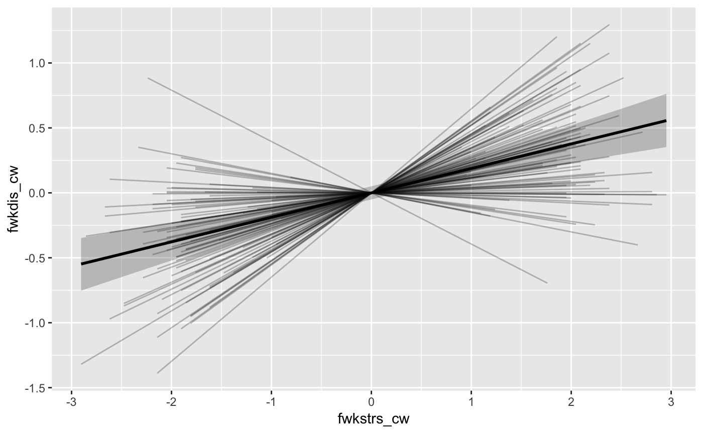
Both plots inside the list ps can be arranged side by
side using the gridExtra package, and can be modified
with the usual ggplot2 functions:
library(ggplot2)
library(gridExtra)
grid.arrange(
    ps[[1]] + labs(title="Path a (X -> M)"),
    ps[[2]] + labs(title="Path b (M -> Y)"),
    nrow=1)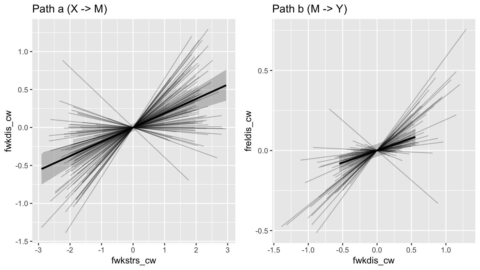
Another example:
ps[[2]] +
    labs(x="Fitted work dissatisfaction",
         y="Fitted relationship dissatisfaction") +
    theme_bw()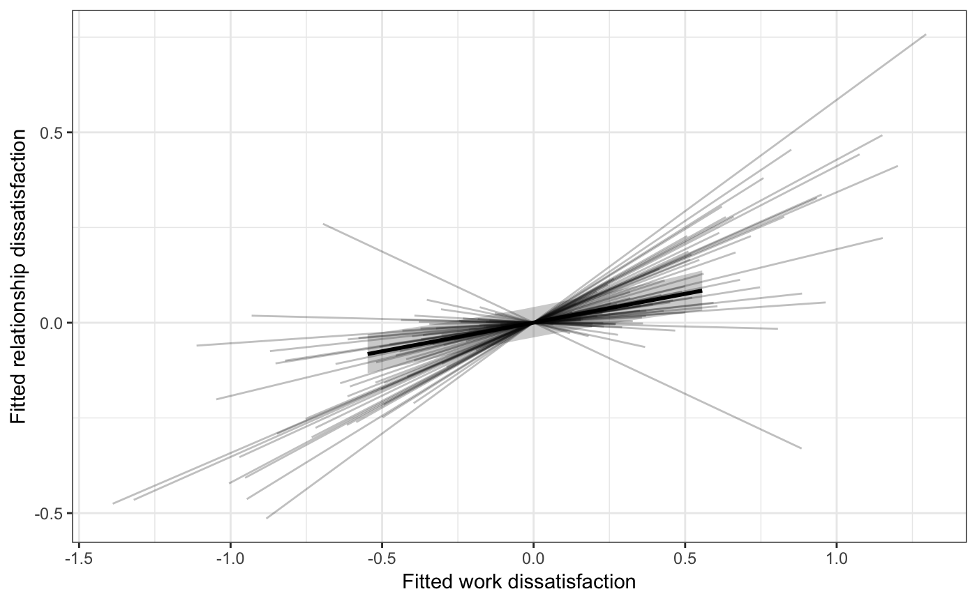
Binary outcome variable
Users can also estimate the multilevel mediation model when the outcome is binary (coded as 0s and 1s). In this case, the outcomes are modelled as bernoulli distributed with a logistic link to the probability parameter of the bernoulli distribution (i.e. the b path is a multilevel logistic regression).
To illustrate, we re-estimate the model using a within person median split Y value as the binary outcome.
library(dplyr)
BLch9_biny <- group_by(BLch9, id) %>%
    select(id, fwkstrs_cw, fwkdis_cw, freldis_cw) %>%
    mutate(biny = as.integer(freldis_cw > quantile(freldis_cw, .5))) %>%
    ungroup()
head(BLch9_biny)
## # A tibble: 6 × 5
## id fwkstrs_cw fwkdis_cw freldis_cw biny
## <int> <dbl> <dbl> <dbl> <int>
## 1 101 0.333 0.983 -1.44 0
## 2 101 0.333 0.928 0.144 0
## 3 101 0.333 -0.719 -1.63 0
## 4 101 1.33 0.745 1.92 1
## 5 101 -1.67 -0.124 -1.93 0
## 6 101 -0.667 -1.27 0.688 1
fit_biny <- mlm(d = BLch9_biny,
                id = "id",
                x = "fwkstrs_cw",
                m = "fwkdis_cw",
                y = "biny", binary_y = TRUE,
                cores=4)
mlm_spaghetti_plot() can also plot fitted values for
models with a binary Y variable.
ps2 <- mlm_spaghetti_plot(fit_biny, BLch9_biny,
                          id="id", x="fwkstrs_cw", m="fwkdis_cw", y="biny",
                          binary_y=T)
The second plot in the list ps2 contains the fitted
values of the b path:
ps2[[2]] + labs(x="Work Dissatisfaction", y="Relationship Dissatisfaction Probability")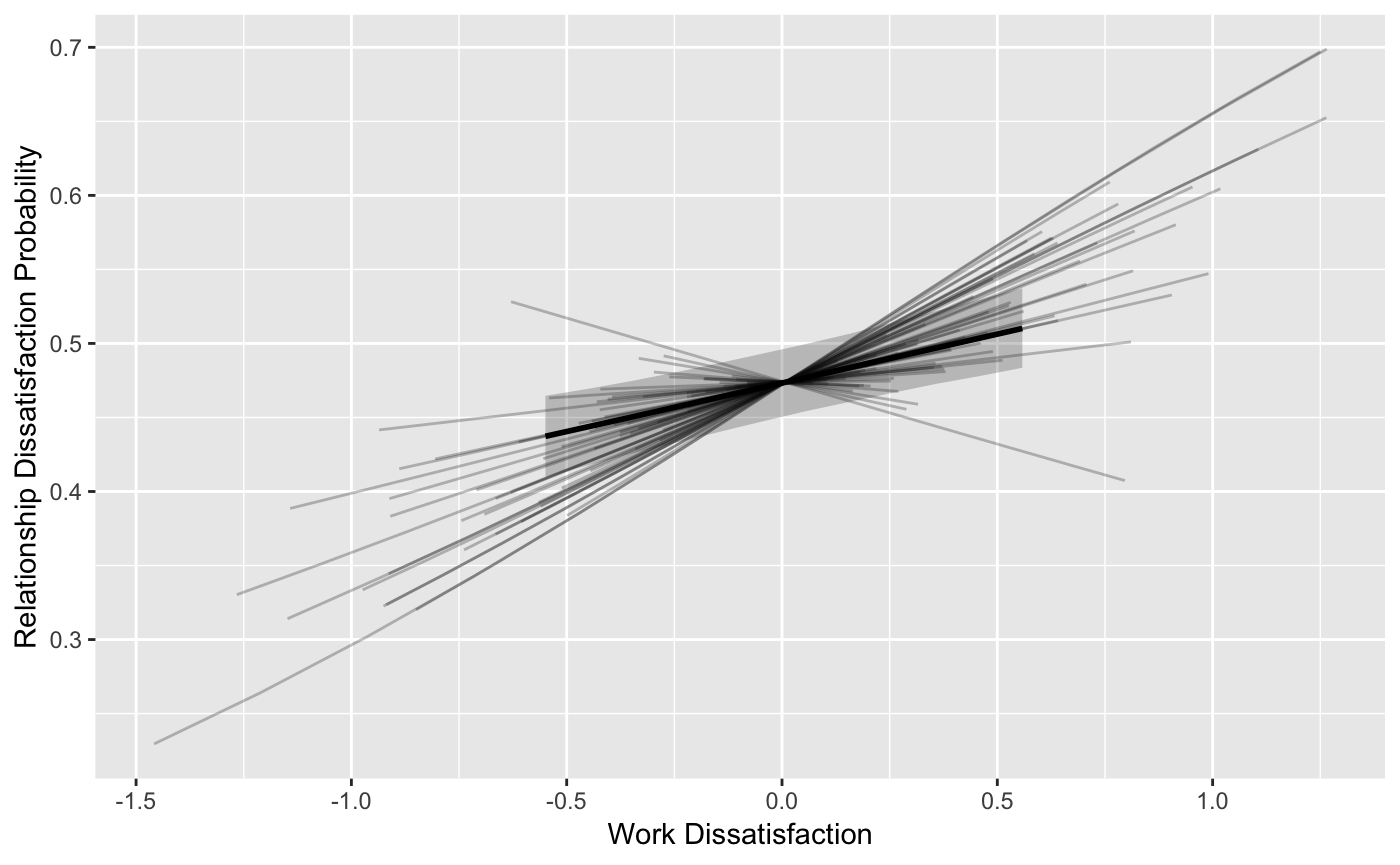
Tips and tricks
Users can investigate person-specific effects by modifying the input to the functions above.
Person-specific effects
It is also possible to investigate person-specific parameters. These exist with the same name as the average-level parameters, but have “u_” appended to them.
head(mlm_summary(fit, pars = "u_c"))## Parameter Mean SE Median 2.5% 97.5% n_eff Rhat
## 1 u_c[1] 0.12 0.08 0.11 -0.02 0.28 3920 1
## 2 u_c[2] 0.10 0.09 0.10 -0.06 0.28 4591 1
## 3 u_c[3] 0.11 0.08 0.10 -0.05 0.29 2838 1
## 4 u_c[4] 0.38 0.13 0.37 0.17 0.67 3224 1
## 5 u_c[5] 0.09 0.09 0.09 -0.11 0.28 4303 1
## 6 u_c[6] 0.08 0.08 0.08 -0.08 0.24 4779 1
mlm_pars_plot(fit, pars = "u_cp", type = "coef", level = .8)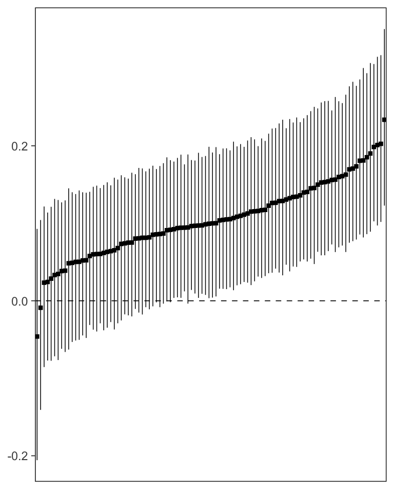
Participant-specific c’ path values with 80% Credible Intervals.
Further information
The functions contained in bmlm have various options available for the user. Inspect these options by looking at the functions’ help pages:
?mlm
?mlm_summary
?mlm_path_plot
?mlm_pars_plot
Users can also input any valid stan() arguments to
mlm(); see ?stan for details. The fitted
object from mlm() is a valid Stanfit object,
so all Stanfit methods are available as well. Functions in
the recent bayesplot package (Gabry, 2016) are supported as well, because the
returned models are Stanfit objects. For example, it is important to
assess the performance of Stan’s MCMC algorithms after estimating a
model by inspecting traceplots for convergence problems:
library(bayesplot)
pars <- c("a", "b", "cp", "corrab")
mcmc_trace(as.data.frame(fit), pars = pars)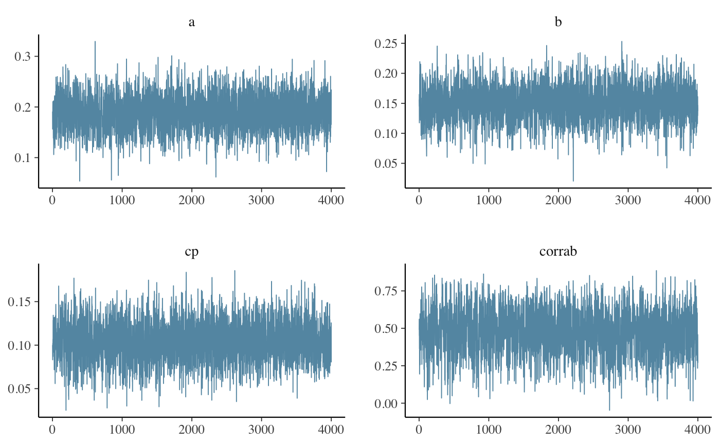
Further modification of the model is possible through modifying the
Stan code underlying mlm().
Citation
If you use this software, please cite it:
citation("bmlm")## To cite package 'bmlm' in publications use:
##
## Vuorre M, Bolger N (2018). "Within-subject mediation analysis for
## experimental data in cognitive psychology and neuroscience."
## _Behavior Research Methods_. doi:10.3758/s13428-017-0980-9
## <https://doi.org/10.3758/s13428-017-0980-9>.
##
## Vuorre M (2023). _bmlm: Bayesian Multilevel Mediation_. R package
## version 1.3.15, <https://CRAN.R-project.org/package=bmlm>.
##
## To see these entries in BibTeX format, use 'print(<citation>,
## bibtex=TRUE)', 'toBibtex(.)', or set
## 'options(citation.bibtex.max=999)'.