A Note on bmlm’s Spaghetti Plots

Matti Vuorre

2023-09-26

library(tidyverse)
library(bmlm)

Consider a mediation model in which Y is binary:

## # A tibble: 6 × 5
##      id      x      m      y  biny
##   <int>  <dbl>  <dbl>  <dbl> <int>
## 1   101  0.333  0.983 -1.44      0
## 2   101  0.333  0.928  0.144     0
## 3   101  0.333 -0.719 -1.63      0
## 4   101  1.33   0.745  1.92      1
## 5   101 -1.67  -0.124 -1.93      0
## 6   101 -0.667 -1.27   0.688     1

fit_biny <- mlm(d = BLch9_biny, 
                id = "id",
                y = "biny", binary_y = TRUE,
                cores=4, iter = 500)

## Warning: The largest R-hat is NA, indicating chains have not mixed.
## Running the chains for more iterations may help. See
## https://mc-stan.org/misc/warnings.html#r-hat

## Warning: Bulk Effective Samples Size (ESS) is too low, indicating posterior means and medians may be unreliable.
## Running the chains for more iterations may help. See
## https://mc-stan.org/misc/warnings.html#bulk-ess

## Warning: Tail Effective Samples Size (ESS) is too low, indicating posterior variances and tail quantiles may be unreliable.
## Running the chains for more iterations may help. See
## https://mc-stan.org/misc/warnings.html#tail-ess

mlm_summary(fit_biny) %>% 
    knitr::kable()

Parameter	Mean	SE	Median	2.5%	97.5%	n_eff	Rhat
a	0.19	0.04	0.19	0.12	0.26	775	1.00
b	0.26	0.05	0.26	0.16	0.37	630	1.01
cp	0.24	0.05	0.24	0.14	0.34	696	1.00
me	0.10	0.03	0.10	0.05	0.15	346	1.01
c	0.34	0.06	0.33	0.22	0.45	660	1.01
pme	0.30	0.08	0.29	0.17	0.46	398	1.01

The mlm_spaghetti_plot() function produces figures in which the horizontal axis values of the M-Y graph (right panel, below) correspond to the vertical axis values of the X-M graph (left panel, below):

pasta <- mlm_spaghetti_plot(fit_biny, BLch9_biny, 
                            id="id", x="x", m="m", y="biny",
                            binary_y=T)
gridExtra::grid.arrange(
    pasta[[1]], 
    pasta[[2]] + coord_cartesian(ylim = 0:1), 
    nrow = 1)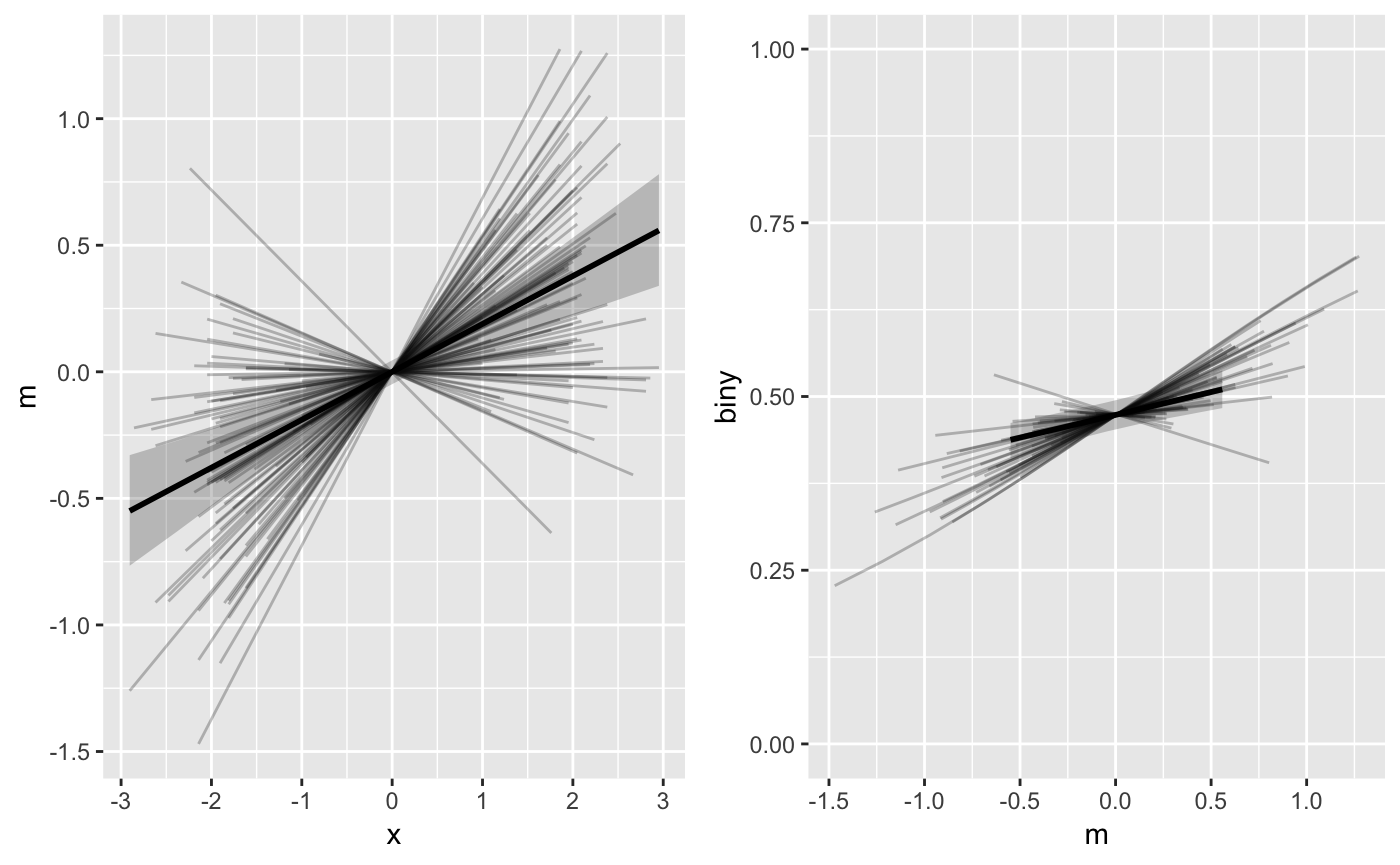

It is important to note that the fitted values (lines) on the right panel of this figure are therefore based on the variation of the fitted values in the left panel, and not on the observed values of m. This behavior usually makes sense and is the default option for mlm_spaghetti_plot(). However, sometimes users may want to plot the M-Y relationship’s (b path’s) fitted values with the observed data values of M on the horizontal axis instead.

To do this, set mx = "data":

pasta2 <- mlm_spaghetti_plot(fit_biny, BLch9_biny, 
                            id="id", x="x", m="m", y="biny",
                            binary_y=T, mx = "data")
gridExtra::grid.arrange(
    pasta2[[1]], 
    pasta2[[2]] + coord_cartesian(ylim = 0:1),
    nrow = 1)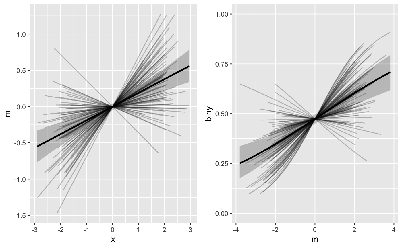

As result, the horizontal axis variability for the b path figure (right panel) is much greater. However, the two panels are no longer directly comparable (vertical axis in left panel doesn’t match horizontal axis of right panel) or interpretable as the model’s implied mediated effect path.

Thanks for reading. Please notify the package’s developer on GitHub if you have further questions or comments.