Data Analysis for V&M (2017)
Matti Vuorre
2017-05-01
library(knitr)
library(gridExtra)
library(lme4)
library(tidyverse)
library(brms)
library(vmapp2017)
knitr::opts_chunk$set(message = F)
Functions and constants
get_pse <- function(X, x, c, scale = 1) {
    # Function to get PSEs
    # X = Matrix of posterior samples (or row of MLEs)
    # x = condition (0 or 1)
    # c = constant (what value ISI is centered on)
    pse <- - ( (X[,1] + X[,3]*x) / (X[,2] + X[,4]*x) )
    pse <- (scale * pse) + c
    return(pse)
}

iters <- 17500
warmups <- 5000
color_vals = c("#e41a1c", "#377eb8")
alphas <- .2

# Estimated models are saved in a local file to save time
load(file="../../../~$models.rda")
Use common plotting theme
library(vmisc)
theme_set(theme_pub())
Data preparation
The data is contained in this package. Here we collapse the illusion data to counts (models estimate faster with collapsed data)
data(illusion)
illusion <- illusion %>%
    group_by(exp, id, condition, cond, interval) %>%
    summarise(k = sum(response, na.rm=T),
              n = n(),
              exclude = unique(exclude)) %>%
    ungroup()
Experiment 1
Apparent Motion
( exp1 <- filter(illusion, exp == 1) )## # A tibble: 384 × 8
## exp id condition cond interval k n exclude
## <chr> <dbl> <chr> <dbl> <dbl> <dbl> <int> <lgl>
## 1 1 101 involuntary 0 33 9 20 FALSE
## 2 1 101 involuntary 0 50 8 20 FALSE
## 3 1 101 involuntary 0 83 8 20 FALSE
## 4 1 101 involuntary 0 100 6 20 FALSE
## 5 1 101 involuntary 0 133 6 20 FALSE
## 6 1 101 involuntary 0 150 5 20 FALSE
## 7 1 101 involuntary 0 200 4 20 FALSE
## 8 1 101 involuntary 0 300 4 20 FALSE
## 9 1 101 voluntary 1 33 10 20 FALSE
## 10 1 101 voluntary 1 50 10 20 FALSE
## # ... with 374 more rows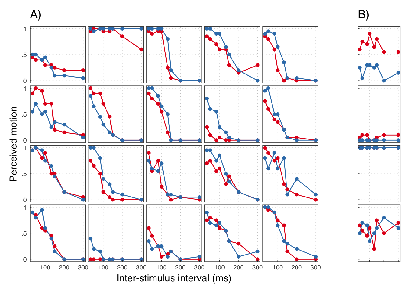
We reject the participants in B.
exp1 <- filter(exp1, exclude == F)
Cc <- mean(unique(exp1$interval))
exp1$isic <- ( exp1$interval - Cc ) / 10
GLMM MLE estimation
exp1mle <- glmer(k/n ~ isic*condition + (isic*condition|id),
                 weights = n, family=binomial(link=logit),
data=exp1)summary(exp1mle)## Generalized linear mixed model fit by maximum likelihood (Laplace
## Approximation) [glmerMod]
## Family: binomial ( logit )
## Formula: k/n ~ isic * condition + (isic * condition | id)
## Data: exp1
## Weights: n
##
## AIC BIC logLik deviance df.resid
## 1256.0 1308.8 -614.0 1228.0 306
##
## Scaled residuals:
## Min 1Q Median 3Q Max
## -2.47676 -0.57691 -0.07241 0.63698 2.81210
##
## Random effects:
## Groups Name Variance Std.Dev. Corr
## id (Intercept) 3.32248 1.8228
## isic 0.01843 0.1358 0.07
## conditionvoluntary 0.51110 0.7149 -0.47 -0.23
## isic:conditionvoluntary 0.02167 0.1472 0.49 -0.24 -0.47
## Number of obs: 320, groups: id, 20
##
## Fixed effects:
## Estimate Std. Error z value Pr(>|z|)
## (Intercept) -1.06610 0.41767 -2.553 0.0107 *
## isic -0.29819 0.03363 -8.868 <2e-16 ***
## conditionvoluntary 0.48399 0.19325 2.504 0.0123 *
## isic:conditionvoluntary -0.01918 0.03860 -0.497 0.6192
## ---
## Signif. codes: 0 '***' 0.001 '**' 0.01 '*' 0.05 '.' 0.1 ' ' 1
##
## Correlation of Fixed Effects:
## (Intr) isic cndtnv
## isic 0.121
## cndtnvlntry -0.475 -0.281
## isc:cndtnvl 0.363 -0.340 -0.189
## convergence code: 0
## Model failed to converge with max|grad| = 0.00229299 (tol = 0.001, component 1)GLMM Bayes estimation
Priors <- c(
    set_prior("normal(0, 100)", class = "b"),
    set_prior("cauchy(0, 4)", class = "sd")
)
exp1b <- brm(k | trials(n) ~ isic*condition + (isic*condition|id),
family=binomial(link=logit), prior = Priors,
data=exp1, cores = 4, iter = iters, warmup = warmups)## Inference for Stan model: binomial(logit) brms-model.
## 4 chains, each with iter=17500; warmup=5000; thin=1;
## post-warmup draws per chain=12500, total post-warmup draws=50000.
##
## mean se_mean sd 2.5% 97.5% n_eff Rhat
## b_Intercept -1.08 0.01 0.49 -2.08 -0.14 8825 1
## b_isic -0.30 0.00 0.04 -0.38 -0.22 17651 1
## b_conditionvoluntary 0.51 0.00 0.23 0.07 0.99 21705 1
## b_isic:conditionvoluntary -0.02 0.00 0.05 -0.12 0.07 22646 1
##
## Samples were drawn using NUTS(diag_e) at Thu Feb 23 10:40:36 2017.
## For each parameter, n_eff is a crude measure of effective sample size,
## and Rhat is the potential scale reduction factor on split chains (at
## convergence, Rhat=1).# Posterior probability (one-sided p-value)
mean(posterior_samples(exp1b, pars = "b_cond") > 0) * 100.0## [1] 98.758Population level PSEs
## # A tibble: 3 × 4
##           key         m       lwr       upr
##         <chr>     <dbl>     <dbl>     <dbl>
## 1  Difference  18.73404  1.809483  37.78756
## 2 Involuntary  94.67529 59.582235 126.39876
## 3   Voluntary 113.40933 84.382228 142.05608
## # A tibble: 3 × 2
## key pp
## <chr> <dbl>
## 1 Difference 0.98334
## 2 Involuntary 0.99986
## 3 Voluntary 1.00000Plot results
e1p4 <- ggplot(exp1psesum, aes(x=reorder(key, rev(m)), m)) +
    geom_hline(yintercept = 0, lty=2) +
    geom_point(size=2) +
    geom_errorbar(aes(ymin=lwr, ymax=upr), width = .2, size=.5) +
    scale_y_continuous("PSE (ms)",
                       breaks = c(-30, 0, 30, 60, 90, 120, 150),
                       limits = c(-35, 155)) +
    scale_x_discrete("Condition",
                     labels = c("Voluntary", "No action", "Difference"))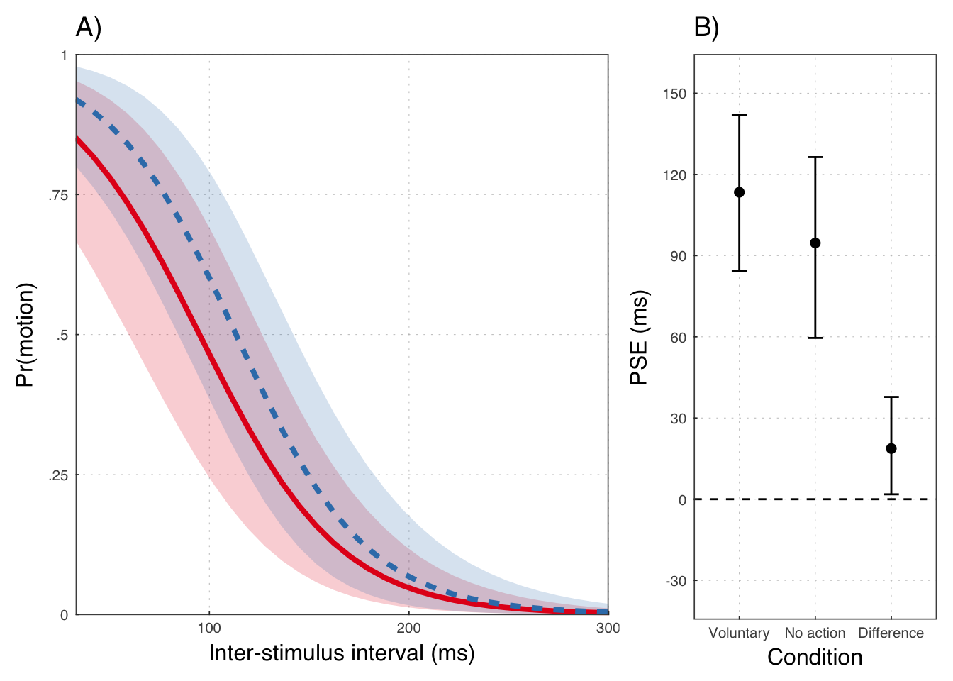
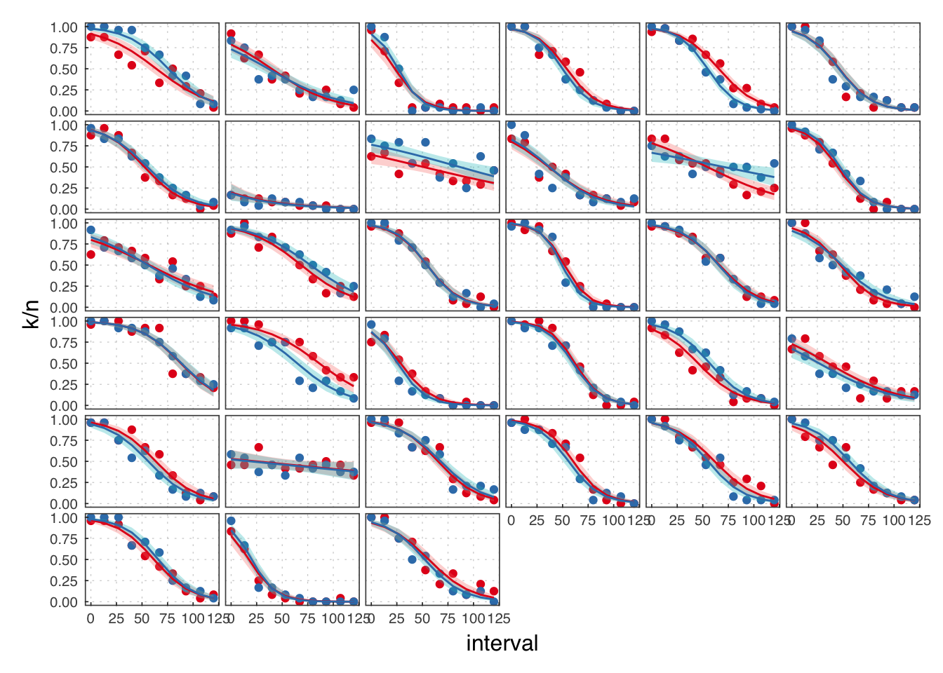
Throughout, we use red to refer to the passive observation condition, and blue to the voluntary action condition.

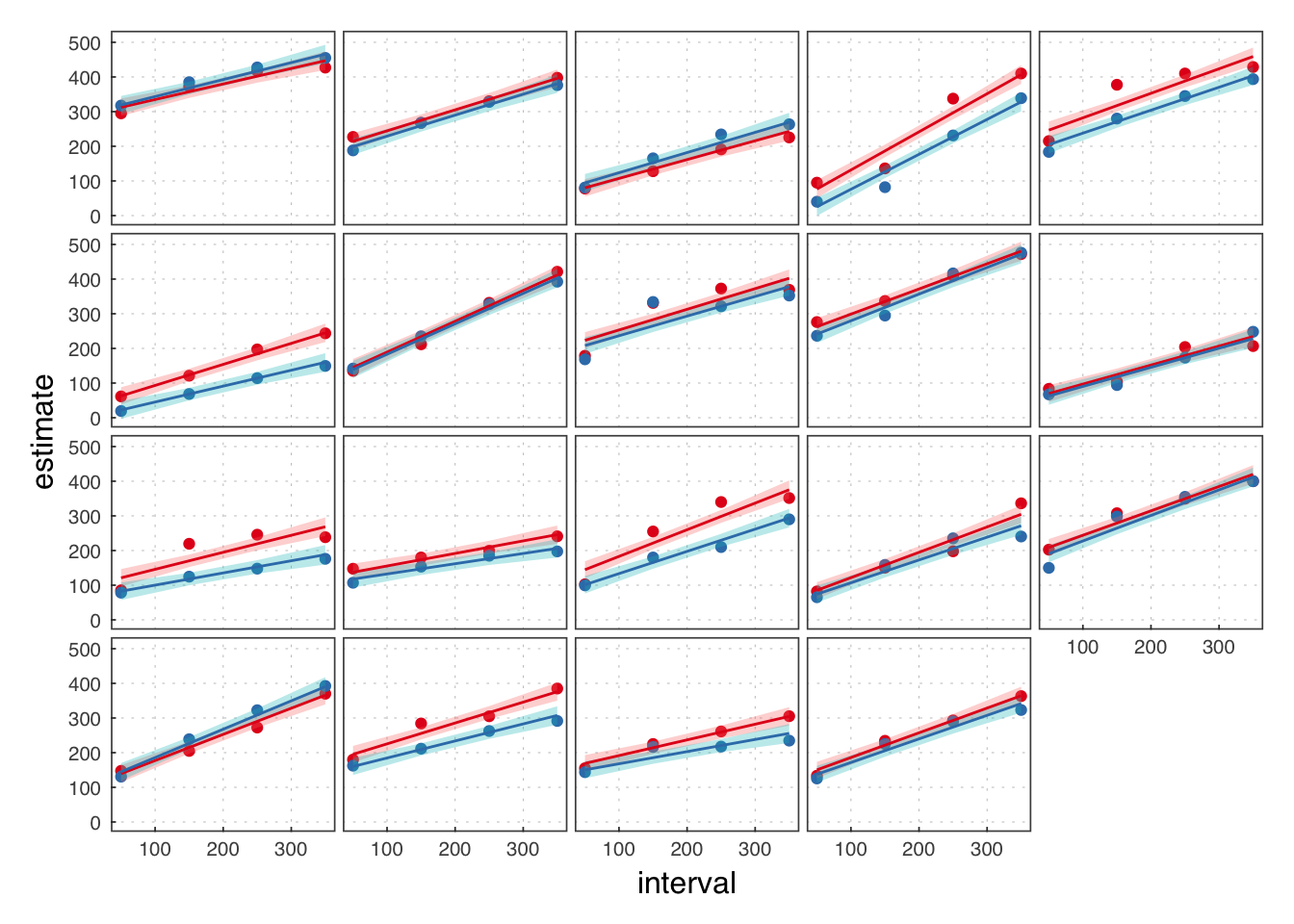
Interval Estimation
data(ie)
ie$isic <- ( ie$interval - mean(unique(ie$interval)) ) / 10
ie
## # A tibble: 3,011 × 6
## id condition interval estimate cond isic
## <dbl> <chr> <int> <dbl> <dbl> <dbl>
## 1 101 voluntary 350 500 1 15
## 2 101 voluntary 250 500 1 5
## 3 101 voluntary 150 400 1 -5
## 4 101 voluntary 150 450 1 -5
## 5 101 voluntary 350 500 1 15
## 6 101 voluntary 250 500 1 5
## 7 101 voluntary 250 450 1 5
## 8 101 voluntary 350 450 1 15
## 9 101 voluntary 50 350 1 -15
## 10 101 voluntary 50 350 1 -15
## # ... with 3,001 more rowsLMM MLE
iemle <- lmerTest::lmer(estimate ~ isic*condition + (isic*condition|id),
data = ie)summary(iemle)## Linear mixed model fit by REML ['merModLmerTest']
## Formula: estimate ~ isic * condition + (isic * condition | id)
## Data: ie
##
## REML criterion at convergence: 35132.8
##
## Scaled residuals:
## Min 1Q Median 3Q Max
## -5.0022 -0.5597 -0.0718 0.4881 5.3010
##
## Random effects:
## Groups Name Variance Std.Dev. Corr
## id (Intercept) 5110.4748 71.4876
## isic 3.3282 1.8243 0.14
## conditionvoluntary 855.9967 29.2574 0.10 -0.28
## isic:conditionvoluntary 0.9201 0.9592 0.35 -0.13 0.96
## Residual 6492.0292 80.5731
## Number of obs: 3011, groups: id, 19
##
## Fixed effects:
## Estimate Std. Error t value
## (Intercept) 257.7719 16.5318 15.593
## isic 6.5033 0.4580 14.200
## conditionvoluntary -25.3937 7.3266 -3.466
## isic:conditionvoluntary -0.3991 0.3428 -1.164
##
## Correlation of Fixed Effects:
## (Intr) isic cndtnv
## isic 0.131
## cndtnvlntry 0.060 -0.234
## isc:cndtnvl 0.223 -0.295 0.567LMM Bayes
ieb <- brm(estimate ~ isic*condition + (isic*condition|id),
           data=ie, cores = 4, iter = iters, warmup = warmups)
## Inference for Stan model: gaussian(identity) brms-model.
## 4 chains, each with iter=17500; warmup=5000; thin=1;
## post-warmup draws per chain=12500, total post-warmup draws=50000.
##
## mean se_mean sd 2.5% 97.5% n_eff Rhat
## b_Intercept 257.78 0.21 19.01 220.03 295.23 8164 1
## b_isic 6.50 0.00 0.52 5.47 7.55 18232 1
## b_conditionvoluntary -25.39 0.05 8.07 -41.37 -9.37 23309 1
## b_isic:conditionvoluntary -0.40 0.00 0.36 -1.10 0.30 50000 1
##
## Samples were drawn using NUTS(diag_e) at Thu Feb 23 10:49:21 2017.
## For each parameter, n_eff is a crude measure of effective sample size,
## and Rhat is the potential scale reduction factor on split chains (at
## convergence, Rhat=1).# Posterior probability (one-sided p-value)
mean(posterior_samples(ieb, pars = "b_cond") < 0) * 100## [1] 99.794Plot results
new_int <- sort(unique(ie$isic))
iepost <- posterior_samples(ieb, pars=parnames(ieb)[1:4])
diffdat <- expand.grid(intrcpt = 0,
                      isic = 0,
                      condition = 1,
                      intrct = new_int)
# create predictor matrix
Xmat <- as.matrix(diffdat)
# matrix for fitted values
fitmat <- matrix(ncol=nrow(iepost), nrow=nrow(diffdat))
# obtain predicted values for each row
for (i in 1:nrow(iepost)) {
    fitmat[,i] <- Xmat %*% as.matrix(iepost)[i,]
}
# get quantiles to plot
diffdat$lower <- apply(fitmat, 1, quantile, prob=0.025)
diffdat$med <- apply(fitmat, 1, quantile, prob=0.5)
diffdat$upper <- apply(fitmat, 1, quantile, prob=0.975)
diffdat$variable <- sort(unique(ie$isic))

e1bp6 <- ggplot(diffdat, aes(x = variable, y=med)) +
    geom_hline(yintercept = 0, lty=2) +
    geom_point(size = 1.4) +
    geom_errorbar(aes(ymin=lower, ymax=upper), width = 1.3, size=.3) +
    scale_y_continuous("Difference (ms)",
                       breaks = c(20, 0, -20, -40, -60, -80),
                       limits = c(-85, 25)) +
    scale_x_continuous("ISI (ms)",
                     breaks = c(-15, -5, 5, 15),
                     labels = c("50", "150", "250", "350"),
                     limits = c(-18, 18))
e1bp7 <- grid.arrange(
e1bp5 +
ggtitle("A)"),
e1bp6 +
ggtitle("B)"),
widths = c(7, 3))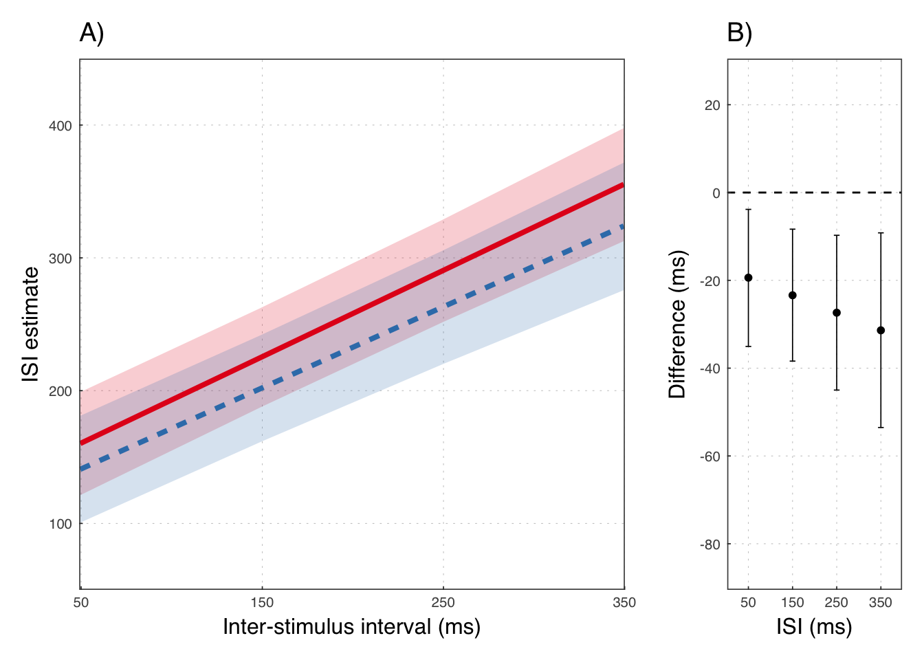
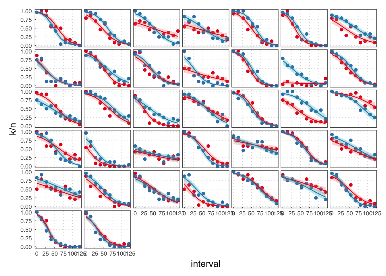
Experiment 2
( exp2 <- filter(illusion, exp == 2) )## # A tibble: 720 × 8
## exp id condition cond interval k n exclude
## <chr> <dbl> <chr> <dbl> <dbl> <dbl> <int> <lgl>
## 1 2 202 involuntary 0 0 17 24 FALSE
## 2 2 202 involuntary 0 13 20 24 FALSE
## 3 2 202 involuntary 0 27 16 24 FALSE
## 4 2 202 involuntary 0 40 19 24 FALSE
## 5 2 202 involuntary 0 53 19 24 FALSE
## 6 2 202 involuntary 0 67 16 24 FALSE
## 7 2 202 involuntary 0 80 13 24 FALSE
## 8 2 202 involuntary 0 93 10 24 FALSE
## 9 2 202 involuntary 0 107 18 24 FALSE
## 10 2 202 involuntary 0 120 7 24 FALSE
## # ... with 710 more rows
We reject the participants in B.
exp2 <- filter(exp2, exclude == F)
Cc <- 50  # ISI to center on (around middle)
exp2$isic <- ( exp2$interval - Cc ) / 10
GLMM MLE estimation
exp2mle <- glmer(k/n ~ isic*condition + (isic*condition|id),
                 weights=n, family=binomial(link=logit),
data=exp2)summary(exp2mle)## Generalized linear mixed model fit by maximum likelihood (Laplace
## Approximation) [glmerMod]
## Family: binomial ( logit )
## Formula: k/n ~ isic * condition + (isic * condition | id)
## Data: exp2
## Weights: n
##
## AIC BIC logLik deviance df.resid
## 2945.7 3008.6 -1458.8 2917.7 646
##
## Scaled residuals:
## Min 1Q Median 3Q Max
## -3.6524 -0.6673 -0.0274 0.7371 3.5086
##
## Random effects:
## Groups Name Variance Std.Dev. Corr
## id (Intercept) 0.91930 0.9588
## isic 0.05073 0.2252 0.64
## conditionvoluntary 0.26396 0.5138 -0.53 -0.41
## isic:conditionvoluntary 0.01289 0.1135 -0.29 -0.45 0.68
## Number of obs: 660, groups: id, 33
##
## Fixed effects:
## Estimate Std. Error z value Pr(>|z|)
## (Intercept) -0.44381 0.17103 -2.595 0.009462 **
## isic -0.50168 0.04127 -12.156 < 2e-16 ***
## conditionvoluntary 0.38996 0.10243 3.807 0.000141 ***
## isic:conditionvoluntary 0.01168 0.02630 0.444 0.656854
## ---
## Signif. codes: 0 '***' 0.001 '**' 0.01 '*' 0.05 '.' 0.1 ' ' 1
##
## Correlation of Fixed Effects:
## (Intr) isic cndtnv
## isic 0.618
## cndtnvlntry -0.527 -0.374
## isc:cndtnvl -0.248 -0.474 0.514GLMM Bayes estimation
exp2b <- brm(k | trials(n) ~ isic*condition + (isic*condition|id),
             family=binomial(link=logit), prior = Priors,
             data=exp2, cores = 4, iter = iters, warmup = warmups)
## Inference for Stan model: binomial(logit) brms-model.
## 4 chains, each with iter=17500; warmup=5000; thin=1;
## post-warmup draws per chain=12500, total post-warmup draws=50000.
##
## mean se_mean sd 2.5% 97.5% n_eff Rhat
## b_Intercept -0.44 0 0.18 -0.79 -0.08 7192 1
## b_isic -0.50 0 0.04 -0.59 -0.42 10762 1
## b_conditionvoluntary 0.38 0 0.11 0.17 0.60 16949 1
## b_isic:conditionvoluntary 0.01 0 0.03 -0.05 0.06 27036 1
##
## Samples were drawn using NUTS(diag_e) at Thu Feb 23 10:53:29 2017.
## For each parameter, n_eff is a crude measure of effective sample size,
## and Rhat is the potential scale reduction factor on split chains (at
## convergence, Rhat=1).# Posterior probability (one-sided p-value)
mean(posterior_samples(exp2b, pars = "b_cond") > 0) * 100## [1] 99.936Population-level PSEs.
## # A tibble: 3 × 4
##           key         m       lwr      upr
##         <chr>     <dbl>     <dbl>    <dbl>
## 1  Difference  7.669065  3.575212 11.93039
## 2 Involuntary 41.370815 35.199276 48.22684
## 3   Voluntary 49.039880 42.937926 56.04192
## # A tibble: 3 × 2
## key pp
## <chr> <dbl>
## 1 Difference 0.9995
## 2 Involuntary 1.0000
## 3 Voluntary 1.0000
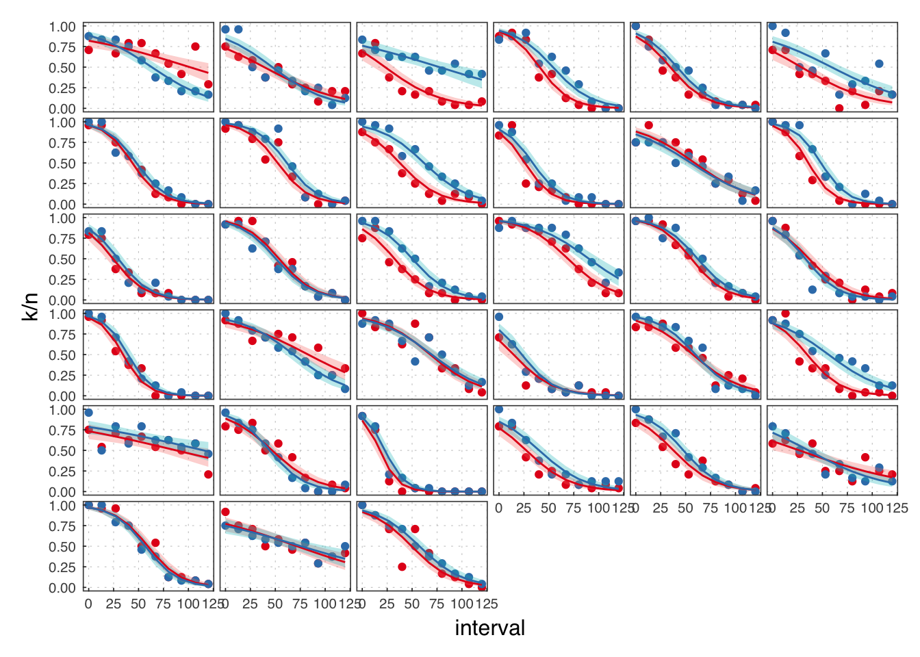
Experiment 3
( exp3 <- filter(illusion, exp == 3) )## # A tibble: 760 × 8
## exp id condition cond interval k n exclude
## <chr> <dbl> <chr> <dbl> <dbl> <dbl> <int> <lgl>
## 1 3 302 involuntary 0 0 23 24 FALSE
## 2 3 302 involuntary 0 13 24 24 FALSE
## 3 3 302 involuntary 0 27 24 24 FALSE
## 4 3 302 involuntary 0 40 13 24 FALSE
## 5 3 302 involuntary 0 53 13 24 FALSE
## 6 3 302 involuntary 0 67 12 24 FALSE
## 7 3 302 involuntary 0 80 4 24 FALSE
## 8 3 302 involuntary 0 93 4 24 FALSE
## 9 3 302 involuntary 0 107 2 24 FALSE
## 10 3 302 involuntary 0 120 0 24 FALSE
## # ... with 750 more rows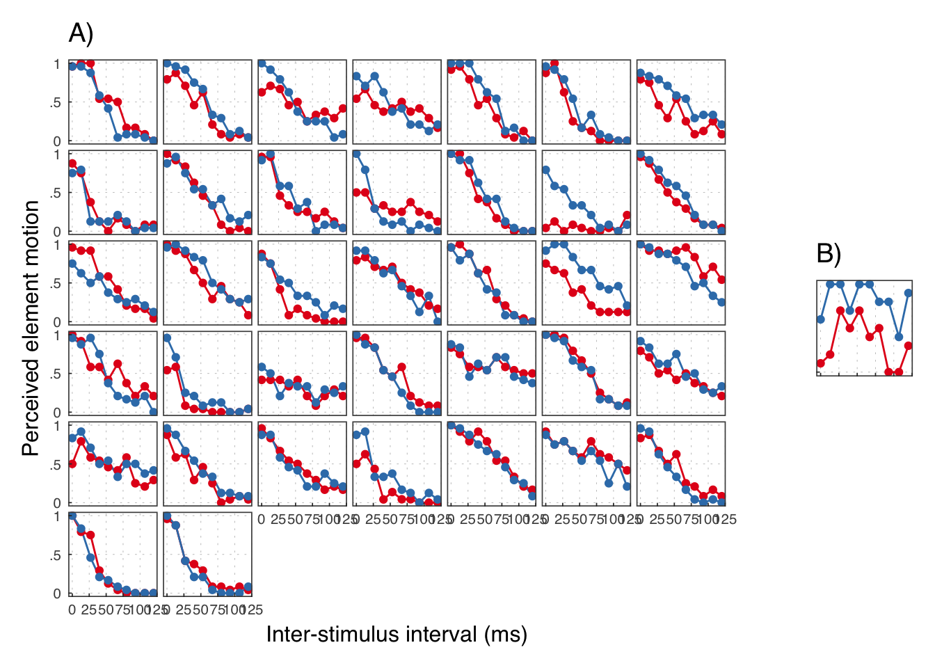
We reject the participants in B.
GLMM MLE estimation
exp3mle <- glmer(k/n ~ isic*condition + (isic*condition|id),
                 weights = n, family=binomial(link=logit),
data=exp3)summary(exp3mle)## Generalized linear mixed model fit by maximum likelihood (Laplace
## Approximation) [glmerMod]
## Family: binomial ( logit )
## Formula: k/n ~ isic * condition + (isic * condition | id)
## Data: exp3
## Weights: n
##
## AIC BIC logLik deviance df.resid
## 3375.7 3440.2 -1673.8 3347.7 726
##
## Scaled residuals:
## Min 1Q Median 3Q Max
## -2.9882 -0.6453 0.0293 0.7307 7.3409
##
## Random effects:
## Groups Name Variance Std.Dev. Corr
## id (Intercept) 0.97817 0.9890
## isic 0.04761 0.2182 0.19
## conditionvoluntary 0.44366 0.6661 -0.62 -0.01
## isic:conditionvoluntary 0.02776 0.1666 -0.08 -0.57 0.19
## Number of obs: 740, groups: id, 37
##
## Fixed effects:
## Estimate Std. Error z value Pr(>|z|)
## (Intercept) -0.25511 0.16570 -1.540 0.1237
## isic -0.40656 0.03737 -10.878 <2e-16 ***
## conditionvoluntary 0.25607 0.11812 2.168 0.0302 *
## isic:conditionvoluntary -0.05164 0.03115 -1.658 0.0973 .
## ---
## Signif. codes: 0 '***' 0.001 '**' 0.01 '*' 0.05 '.' 0.1 ' ' 1
##
## Correlation of Fixed Effects:
## (Intr) isic cndtnv
## isic 0.184
## cndtnvlntry -0.618 -0.023
## isc:cndtnvl -0.075 -0.576 0.164
## convergence code: 0
## Model failed to converge with max|grad| = 0.00147215 (tol = 0.001, component 1)GLMM Bayes estimation
exp3b <- brm(k | trials(n) ~ isic*condition + (isic*condition|id),
             family=binomial(link=logit), prior = Priors,
             data=exp3, cores = 4, iter = iters, warmup = warmups)
## Inference for Stan model: binomial(logit) brms-model.
## 4 chains, each with iter=17500; warmup=5000; thin=1;
## post-warmup draws per chain=12500, total post-warmup draws=50000.
##
## mean se_mean sd 2.5% 97.5% n_eff Rhat
## b_Intercept -0.248 0.002 0.178 -0.598 0.101 6657 1
## b_isic -0.405 0.000 0.040 -0.486 -0.328 9487 1
## b_conditionvoluntary 0.253 0.001 0.127 0.002 0.503 10594 1
## b_isic:conditionvoluntary -0.055 0.000 0.033 -0.120 0.012 15592 1
##
## Samples were drawn using NUTS(diag_e) at Thu Feb 23 10:58:10 2017.
## For each parameter, n_eff is a crude measure of effective sample size,
## and Rhat is the potential scale reduction factor on split chains (at
## convergence, Rhat=1).# Posterior probability (one-sided p-value)
mean(posterior_samples(exp3b, pars = "b_cond") > 0) * 100## [1] 97.574## # A tibble: 3 × 4
## key m lwr upr
## <chr> <dbl> <dbl> <dbl>
## 1 Difference 6.281609 0.1284105 12.65075
## 2 Involuntary 43.905706 35.2922935 52.56462
## 3 Voluntary 50.187315 43.9534229 56.85072## # A tibble: 3 × 2
## key pp
## <chr> <dbl>
## 1 Difference 0.9772
## 2 Involuntary 1.0000
## 3 Voluntary 1.0000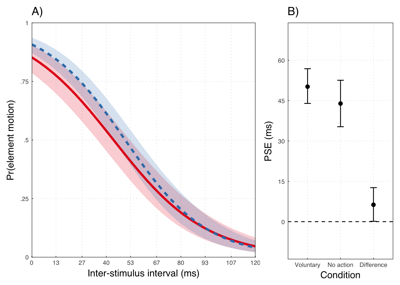
Experiment 4
( exp4 <- filter(illusion, exp == 4) )## # A tibble: 720 × 8
## exp id condition cond interval k n exclude
## <chr> <dbl> <chr> <dbl> <dbl> <dbl> <int> <lgl>
## 1 4 403 no_warning 0 0 21 24 FALSE
## 2 4 403 no_warning 0 13 21 24 FALSE
## 3 4 403 no_warning 0 27 16 24 FALSE
## 4 4 403 no_warning 0 40 13 24 FALSE
## 5 4 403 no_warning 0 53 17 24 FALSE
## 6 4 403 no_warning 0 67 8 24 FALSE
## 7 4 403 no_warning 0 80 12 24 FALSE
## 8 4 403 no_warning 0 93 7 24 FALSE
## 9 4 403 no_warning 0 107 5 24 FALSE
## 10 4 403 no_warning 0 120 1 24 FALSE
## # ... with 710 more rows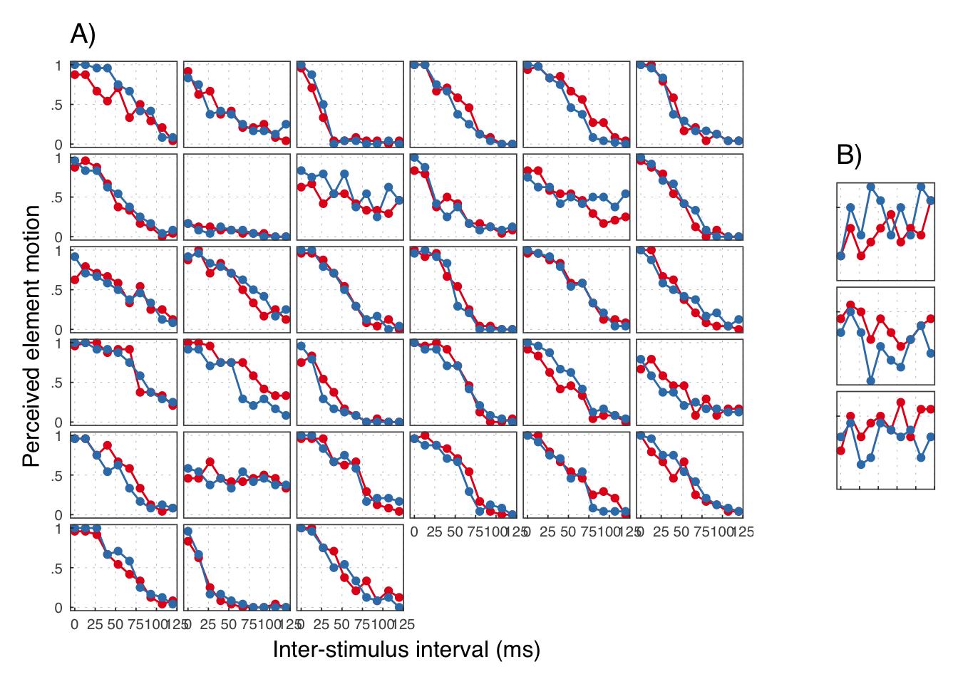
We reject the participants in B.
GLMM MLE estimation
exp4mle <- glmer(k/n ~ isic*condition + (isic*condition|id),
                 weights = n, family=binomial(link=logit),
data=exp4)summary(exp4mle)## Generalized linear mixed model fit by maximum likelihood (Laplace
## Approximation) [glmerMod]
## Family: binomial ( logit )
## Formula: k/n ~ isic * condition + (isic * condition | id)
## Data: exp4
## Weights: n
##
## AIC BIC logLik deviance df.resid
## 2815.3 2878.2 -1393.6 2787.3 646
##
## Scaled residuals:
## Min 1Q Median 3Q Max
## -2.6876 -0.6251 0.0345 0.7519 7.0223
##
## Random effects:
## Groups Name Variance Std.Dev. Corr
## id (Intercept) 0.959136 0.9794
## isic 0.038146 0.1953 0.02
## conditionwarning 0.137033 0.3702 -0.07 0.23
## isic:conditionwarning 0.008463 0.0920 0.19 0.15 0.06
## Number of obs: 660, groups: id, 33
##
## Fixed effects:
## Estimate Std. Error z value Pr(>|z|)
## (Intercept) 0.03681 0.17399 0.212 0.832
## isic -0.49405 0.03601 -13.721 <2e-16 ***
## conditionwarning -0.02879 0.08109 -0.355 0.723
## isic:conditionwarning -0.02762 0.02347 -1.177 0.239
## ---
## Signif. codes: 0 '***' 0.001 '**' 0.01 '*' 0.05 '.' 0.1 ' ' 1
##
## Correlation of Fixed Effects:
## (Intr) isic cndtnw
## isic 0.015
## condtnwrnng -0.138 0.178
## isc:cndtnwr 0.134 -0.065 0.037table(exp4$id)##
## 403 404 405 406 407 408 409 410 411 412 413 416 417 418 419 420 421 422
## 20 20 20 20 20 20 20 20 20 20 20 20 20 20 20 20 20 20
## 423 424 425 426 428 429 430 431 432 433 434 435 436 437 438
## 20 20 20 20 20 20 20 20 20 20 20 20 20 20 20GLMM Bayes estimation
exp4b <- brm(k | trials(n) ~ isic*condition + (isic*condition|id),
             family=binomial(link=logit), prior = Priors,
             data=exp4, cores = 4, iter = iters, warmup = warmups)
## Inference for Stan model: binomial(logit) brms-model.
## 4 chains, each with iter=17500; warmup=5000; thin=1;
## post-warmup draws per chain=12500, total post-warmup draws=50000.
##
## mean se_mean sd 2.5% 97.5% n_eff Rhat
## b_Intercept 0.035 0.002 0.194 -0.346 0.414 6430 1
## b_isic -0.495 0.000 0.040 -0.575 -0.418 11964 1
## b_conditionwarning -0.026 0.001 0.089 -0.202 0.148 25845 1
## b_isic:conditionwarning -0.027 0.000 0.025 -0.077 0.021 33775 1
##
## Samples were drawn using NUTS(diag_e) at Thu Feb 23 11:01:35 2017.
## For each parameter, n_eff is a crude measure of effective sample size,
## and Rhat is the potential scale reduction factor on split chains (at
## convergence, Rhat=1).# Posterior probability (one-sided p-value)
mean(posterior_samples(exp4b, pars = "b_cond") > 0) * 100## [1] 38.34## # A tibble: 3 × 2
## key pp
## <chr> <dbl>
## 1 Difference 0.38266
## 2 No Warning 1.00000
## 3 Warning 1.00000## # A tibble: 3 × 4
## key m lwr upr
## <chr> <dbl> <dbl> <dbl>
## 1 Difference -0.4917079 -3.880532 2.976048
## 2 No Warning 50.7151923 42.981034 58.508879
## 3 Warning 50.2234844 42.574335 58.167847
Combined analysis
We also compared the effect of condition across the Ternus experiments using an interaction term. That is, is the effect of condition greater in experiments 2 and 3, than in experiment 4?
( fulldata <- illusion %>% filter(exp > 1, !exclude) )## # A tibble: 2,060 × 8
## exp id condition cond interval k n exclude
## <chr> <dbl> <chr> <dbl> <dbl> <dbl> <int> <lgl>
## 1 2 202 involuntary 0 0 17 24 FALSE
## 2 2 202 involuntary 0 13 20 24 FALSE
## 3 2 202 involuntary 0 27 16 24 FALSE
## 4 2 202 involuntary 0 40 19 24 FALSE
## 5 2 202 involuntary 0 53 19 24 FALSE
## 6 2 202 involuntary 0 67 16 24 FALSE
## 7 2 202 involuntary 0 80 13 24 FALSE
## 8 2 202 involuntary 0 93 10 24 FALSE
## 9 2 202 involuntary 0 107 18 24 FALSE
## 10 2 202 involuntary 0 120 7 24 FALSE
## # ... with 2,050 more rowsfulldata$isic <- ( fulldata$interval - Cc ) / 10GLMM MLE Estimation
fullmle <- glmer(k/n ~ isic*cond + exp*isic + exp*cond +
                     (isic*cond|id),
                 weights=n, family=binomial(link=logit),
                 data=fulldata)
## Warning in checkConv(attr(opt, "derivs"), opt$par, ctrl = control
## $checkConv, : Model failed to converge with max|grad| = 0.0114011 (tol =
## 0.001, component 1)summary(fullmle)## Generalized linear mixed model fit by maximum likelihood (Laplace
## Approximation) [glmerMod]
## Family: binomial ( logit )
## Formula: k/n ~ isic * cond + exp * isic + exp * cond + (isic * cond |
## id)
## Data: fulldata
## Weights: n
##
## AIC BIC logLik deviance df.resid
## 9130.2 9242.8 -4545.1 9090.2 2040
##
## Scaled residuals:
## Min 1Q Median 3Q Max
## -3.6651 -0.6525 0.0077 0.7289 7.1248
##
## Random effects:
## Groups Name Variance Std.Dev. Corr
## id (Intercept) 0.93472 0.9668
## isic 0.04454 0.2110 0.27
## cond 0.27952 0.5287 -0.45 -0.07
## isic:cond 0.01699 0.1304 -0.05 -0.36 0.26
## Number of obs: 2060, groups: id, 103
##
## Fixed effects:
## Estimate Std. Error z value Pr(>|z|)
## (Intercept) -0.41374 0.17236 -2.400 0.016377 *
## isic -0.48214 0.03644 -13.230 < 2e-16 ***
## cond 0.35137 0.10233 3.434 0.000595 ***
## exp3 0.15485 0.23977 0.646 0.518390
## exp4 0.44358 0.24301 1.825 0.067947 .
## isic:cond -0.02398 0.01595 -1.504 0.132697
## isic:exp3 0.06101 0.04922 1.240 0.215137
## isic:exp4 -0.01421 0.04996 -0.284 0.776073
## cond:exp3 -0.07537 0.14043 -0.537 0.591464
## cond:exp4 -0.37480 0.14341 -2.613 0.008962 **
## ---
## Signif. codes: 0 '***' 0.001 '**' 0.01 '*' 0.05 '.' 0.1 ' ' 1
##
## Correlation of Fixed Effects:
## (Intr) isic cond exp3 exp4 isc:cn isc:x3 isc:x4 cnd:x3
## isic 0.267
## cond -0.450 -0.015
## exp3 -0.728 -0.188 0.317
## exp4 -0.708 -0.185 0.317 0.514
## isic:cond -0.022 -0.222 0.134 -0.018 0.004
## isic:exp3 -0.195 -0.705 -0.019 0.269 0.137 -0.038
## isic:exp4 -0.189 -0.687 -0.010 0.137 0.263 -0.006 0.514
## cond:exp3 0.332 -0.009 -0.724 -0.455 -0.234 -0.008 0.016 0.007
## cond:exp4 0.323 -0.005 -0.697 -0.235 -0.457 -0.020 0.009 0.017 0.511
## convergence code: 0
## Model failed to converge with max|grad| = 0.0114011 (tol = 0.001, component 1)GLMM Bayes estimation
fullb <- brm(k | trials(n) ~ isic*cond + exp*isic + exp*cond +
                 (isic*cond|id),
             family=binomial(link=logit), prior = Priors,
             data=fulldata, cores = 4, iter = iters, warmup = warmups,
             save_ranef = FALSE)  # Save space
## Family: binomial(logit)
## Formula: k | trials(n) ~ isic * cond + exp * isic + exp * cond + (isic * cond | id)
## Data: fulldata (Number of observations: 2060)
## Samples: 4 chains, each with iter = 17500; warmup = 5000; thin = 1;
## total post-warmup samples = 50000
## WAIC: Not computed
##
## Group-Level Effects:
## ~id (Number of levels: 103)
## Estimate Est.Error l-95% CI u-95% CI Eff.Sample
## sd(Intercept) 1.00 0.08 0.86 1.17 11235
## sd(isic) 0.22 0.02 0.19 0.26 12578
## sd(cond) 0.55 0.05 0.46 0.66 17779
## sd(isic:cond) 0.13 0.01 0.11 0.16 20396
## cor(Intercept,isic) 0.26 0.10 0.05 0.45 9725
## cor(Intercept,cond) -0.43 0.10 -0.60 -0.22 21907
## cor(isic,cond) -0.05 0.12 -0.28 0.18 14458
## cor(Intercept,isic:cond) -0.03 0.13 -0.28 0.22 19748
## cor(isic,isic:cond) -0.33 0.11 -0.54 -0.09 20461
## cor(cond,isic:cond) 0.24 0.13 -0.02 0.48 15893
## Rhat
## sd(Intercept) 1
## sd(isic) 1
## sd(cond) 1
## sd(isic:cond) 1
## cor(Intercept,isic) 1
## cor(Intercept,cond) 1
## cor(isic,cond) 1
## cor(Intercept,isic:cond) 1
## cor(isic,isic:cond) 1
## cor(cond,isic:cond) 1
##
## Population-Level Effects:
## Estimate Est.Error l-95% CI u-95% CI Eff.Sample Rhat
## Intercept -0.41 0.18 -0.77 -0.06 4998 1
## isic -0.48 0.04 -0.55 -0.41 8096 1
## cond 0.35 0.11 0.15 0.56 10047 1
## exp3 0.16 0.25 -0.33 0.64 4592 1
## exp4 0.45 0.25 -0.05 0.94 4750 1
## isic:cond -0.03 0.02 -0.06 0.01 23692 1
## isic:exp3 0.06 0.05 -0.04 0.16 7519 1
## isic:exp4 -0.02 0.05 -0.12 0.09 8059 1
## cond:exp3 -0.08 0.14 -0.36 0.21 9778 1
## cond:exp4 -0.38 0.15 -0.67 -0.08 10662 1
##
## Samples were drawn using sampling(NUTS). For each parameter, Eff.Sample
## is a crude measure of effective sample size, and Rhat is the potential
## scale reduction factor on split chains (at convergence, Rhat = 1).Posterior probability that effect of condition (i.e. warning condition effect is smaller than voluntary action condition effect).
# Posterior probability (one-sided p-value)
mean(posterior_samples(fullb, pars = "b_cond:exp4") < 0) * 100
## [1] 99.4Compare effect of condition across the three Ternus experiments:
x <- as.data.frame(fullb, pars = "b_cond") %>%
    as_tibble() %>%
    transmute(cond_exp2 = b_cond,
              cond_exp3 = b_cond + b_cond.exp3,
              cond_exp4 = b_cond + b_cond.exp4,
              cond_2v3 = b_cond.exp3,
              cond_2v4 = b_cond.exp4,
              cond_3v4 = cond_exp4 - cond_exp3)
x %>%
    gather() %>%
    group_by(key) %>%
    summarize(bhat = mean(value),
              `2.5%ile` = quantile(value, probs = 0.025),
              `97.5%ile` = quantile(value, probs = 0.975))
## # A tibble: 6 × 4
## key bhat `2.5%ile` `97.5%ile`
## <chr> <dbl> <dbl> <dbl>
## 1 cond_2v3 -0.07702028 -0.36268402 0.20589888
## 2 cond_2v4 -0.37716975 -0.67038813 -0.08425850
## 3 cond_3v4 -0.30014947 -0.58698900 -0.01374827
## 4 cond_exp2 0.35233824 0.14620466 0.56059514
## 5 cond_exp3 0.27531796 0.07914614 0.47232450
## 6 cond_exp4 -0.02483151 -0.23728027 0.18591864