Forest plots for brmsfit models with varying effects

Matti Vuorre

2018-10-19

library(here)
library(brms)
library(brmstools)
library(dplyr)

Introduction

Forest plots display estimated parameters from multiple sources (studies, participants, etc.) in one figure. They are most commonly used in meta-analysis, where individual studies are used to inform an average, or meta-analytic, overall estimate. However, they can be seamlessly applied to other types of multilevel models–models in which parameters are assumed to vary among units. brmstools’ forest() function draws forest plots from brmsfit objects. They should be most useful for meta-analytic models, but can be produced from any brmsfit with one or more varying parameters.

The forest() function uses the fantastic ggridges R package in the backend, and assumes you’ve installed it. If you haven’t, forest() will return an error.

Random effects meta-analysis

We illustrate using a data set from the metafor package.

data("dat.bangertdrowns2004", package = "metafor")
dat <- dat.bangertdrowns2004 %>%
  mutate(study = paste0(author, " (", year, ")"), sei = sqrt(vi)) %>%
  select(study, yi, sei) %>%
  slice(1:15)

brms allows flexible specification of meta-analytic models.

fit_rem <- brm(
  yi | se(sei) ~ 1 + (1|study),
  data = dat,
  cores = 4, 
  control=list(adapt_delta = .99)
)

Use forest() to draw the forest plot:

forest(fit_rem)
#> Picking joint bandwidth of 0.0227

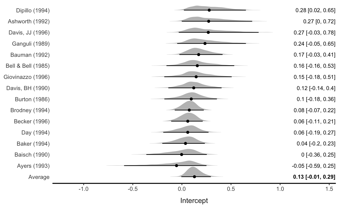
There are various options (see ?forest)

forest(fit_rem, 
       level = .80, 
       av_name = "Meta-Analytic\nEstimate", 
       col_ridge = "purple", 
       fill_ridge = "grey90")
#> Picking joint bandwidth of 0.0227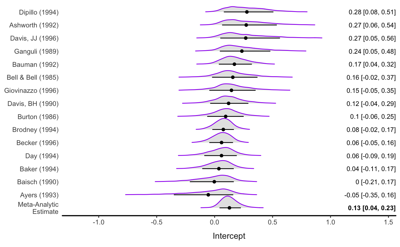

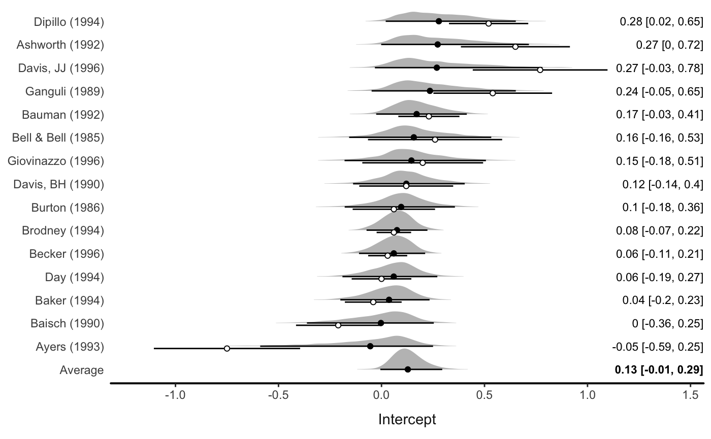
Data points can also be shown (note this probably only makes sense with a meta-analytic model):

forest(fit_rem, show_data = T)
#> Joining, by = "study"
#> Picking joint bandwidth of 0.0227

Multilevel model

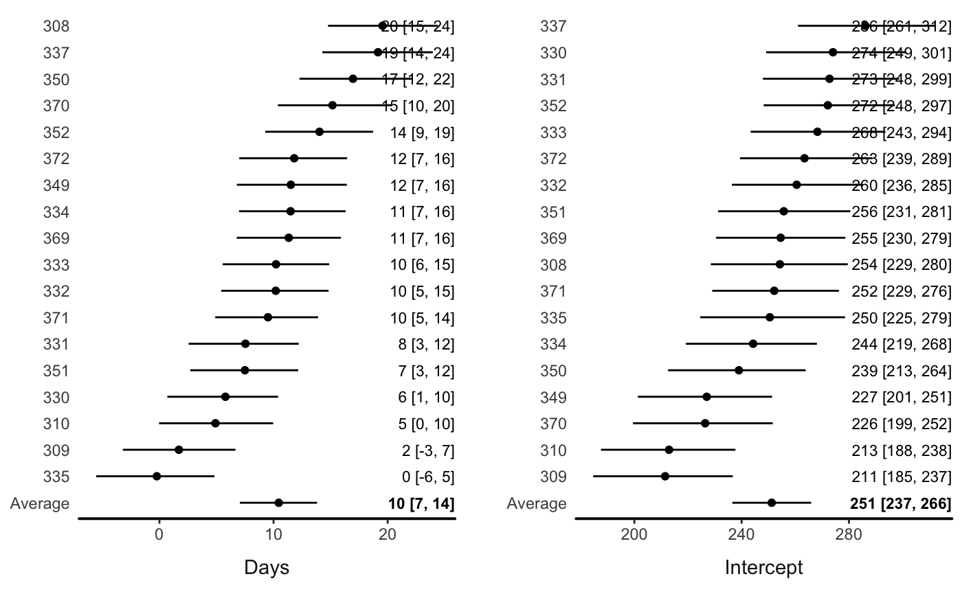
The forest() function can be seamlessly applied to any multilevel model.

We use example data from the lme4 package.

data(sleepstudy, package = "lme4")
head(sleepstudy)
#>   Reaction Days Subject
#> 1 249.5600    0     308
#> 2 258.7047    1     308
#> 3 250.8006    2     308
#> 4 321.4398    3     308
#> 5 356.8519    4     308
#> 6 414.6901    5     308

A multilevel model with varying intercepts and slopes (effect of Days):

fit_ml <- brm(
  Reaction ~ Days + (Days|Subject),
  data = sleepstudy,
  cores = 4
)

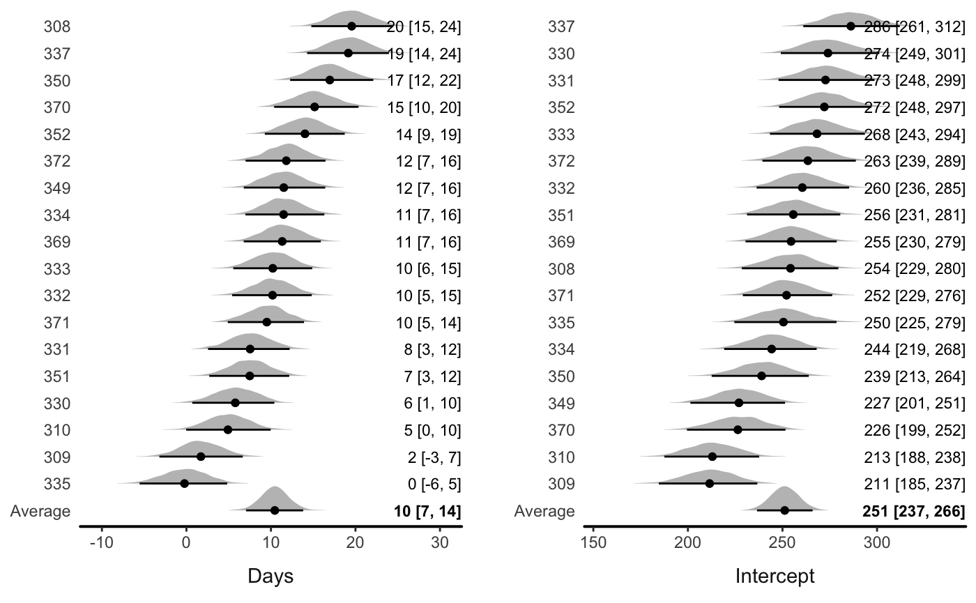
If there are multiple varying parameters, users can input a variable name:

forest(fit_ml, pars = "Days")
#> Picking joint bandwidth of 0.41

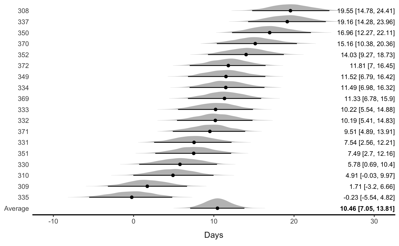
Or let the function automatically draw a plot with all the variables:

forest(fit_ml, digits=0)
#> Picking joint bandwidth of 0.41
#> Picking joint bandwidth of 2.15

You can also turn off the ridgeline plots (densities)

forest(fit_ml, density = F, digits=0)