Coefficient plots

Matti Vuorre

2018-10-18

library(here)
library(brms)
library(brmstools)
library(dplyr)

head(fit_ml$data)
#>   Reaction Days Subject
#> 1 249.5600    0     308
#> 2 258.7047    1     308
#> 3 250.8006    2     308
#> 4 321.4398    3     308
#> 5 356.8519    4     308
#> 6 414.6901    5     308

summary(fit_ml)
#>  Family: gaussian 
#>   Links: mu = identity; sigma = identity 
#> Formula: Reaction ~ Days + (Days | Subject) 
#>    Data: sleepstudy (Number of observations: 180) 
#> Samples: 4 chains, each with iter = 2000; warmup = 1000; thin = 1;
#>          total post-warmup samples = 4000
#> 
#> Group-Level Effects: 
#> ~Subject (Number of levels: 18) 
#>                     Estimate Est.Error l-95% CI u-95% CI Eff.Sample Rhat
#> sd(Intercept)          26.67      6.78    15.38    42.84       1595 1.00
#> sd(Days)                6.54      1.51     4.12     9.89       1254 1.00
#> cor(Intercept,Days)     0.10      0.30    -0.48     0.69        918 1.00
#> 
#> Population-Level Effects: 
#>           Estimate Est.Error l-95% CI u-95% CI Eff.Sample Rhat
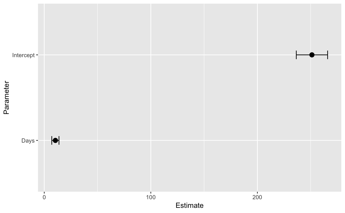
#> Intercept   251.19      7.47   236.52   265.91       1850 1.00
#> Days         10.46      1.70     7.05    13.81       1525 1.00
#> 
#> Family Specific Parameters: 
#>       Estimate Est.Error l-95% CI u-95% CI Eff.Sample Rhat
#> sigma    25.92      1.54    23.09    29.09       3140 1.00
#> 
#> Samples were drawn using sampling(NUTS). For each parameter, Eff.Sample 
#> is a crude measure of effective sample size, and Rhat is the potential 
#> scale reduction factor on split chains (at convergence, Rhat = 1).

Coefficient plots

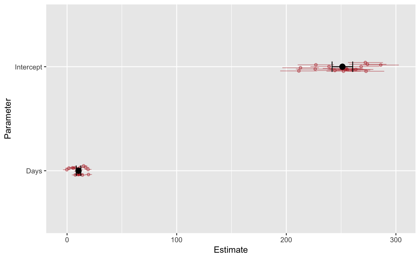
A coefficient plot is a visual replacement of a table summarizing a fitted model’s parameters. brmstools’ coefplot() draws population-level and group-specific parameter means and credible intervals on the same plot.

coefplot(fit_ml, 
         level = .8,
         r_intervals = TRUE, 
         r_col = "firebrick")

Users can plot a single parameter by naming it:

coefplot(fit_ml, pars = "Days", r_intervals = T)

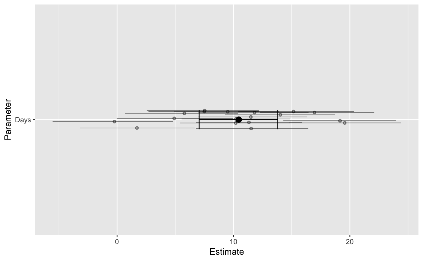
Or only the population-level / group-specific parameters:

coefplot(fit_ml, type = "b")